

A common misperception in investing is that “over diversified” portfolios lead to lower returns. This is wrong. This fallacy leads many investors to assume greater investment risk than necessary, which reduces wealth over time. At Mercer Advisors, we think a lot about what clients pay (risk) for what they get in return (compound returns). Broad diversification is the key to help ensure investors don’t overpay, and it is a fundamental driver of long-term Economic Freedom™.
This piece explores why.
Over the past century, only 4% of all stocks that were ever publicly traded account for all of the net wealth created in the U.S. stock market.1 Further, and perhaps more shocking, over half of all publicly traded stocks (59%) over the past 100 years failed to outperform the return on a one-month U.S. Treasury bill.2 Over time, wealth creation has become even more concentrated among fewer firms.
For most investors, U.S. large company stocks typically make up the single largest asset allocation within their portfolios. (For purposes of our discussion, we focus primarily on the US stock market. But the principles we discuss throughout this article are equally applicable to virtually all assets.)
The challenge for such investors is threefold: it is not possible to reliably predict which stocks will generate long-term wealth; holding a concentrated position in a single stock is more risky, on average, than the broader market; and volatility is extremely costly to investors because it drags down the long-run compound return.3
We argue that diversification provides three primary benefits.
- First, it helps reduce risk (portfolio volatility).
- Second, by lowering portfolio volatility, diversification may increase compound returns over time.
- Finally, diversification is a strategy designed to maximize our odds of successfully building and sustaining wealth over time.
Together, these benefits make diversification one of the most reliable and powerful tools available to investors.
Understanding the problem: When 8% is not 8%
Most investors appreciate that it is riskier to hold a single stock than a broadly diversified portfolio. It is less widely appreciated that, over the long run, the typical individual stock generates a lower compound return than the broad market or specific asset class to which it belongs.
The compound return (or geometric return) measures the rate at which wealth compounds over time. These are the returns that matter. It is not the same as the arithmetic average return, and the difference between the two can be substantial.
Consider a portfolio that gains 20% in one year and loses 20% in the next. The arithmetic average return is 0%, because the gain and loss offset one another. Yet the investor does not end up where they started. A $100,000 portfolio grows to $120,000 after the first year but falls to $96,000 after the second. Despite an average return of zero, the investor has lost $4,000. The greater the volatility, the larger this gap becomes.
The difference between the arithmetic and compound return is known as volatility drag and is the hidden cost that volatility (risk) steals from long-term wealth accumulation. As the volatility of a portfolio increases, the compound return declines exponentially. For example, a portfolio with a 20% volatility loses approximately 2.0 percentage points per year to the volatility drag, while a portfolio with a 10% volatility loses 0.5 percentage points per year (see Appendix 1). The resulting 1.5 percentage point advantage is captured simply by holding a less volatile, more diversified portfolio.
Figure 1 illustrates the wealth effect of three portfolios that share the same expected arithmetic return of 8% but have very different levels of volatility: 10%, 20%, and 30%. Although all three portfolios have identical expected returns, their long-term wealth outcomes differ dramatically because of volatility drag. After 30 years, a $100,000 investment in the portfolio with 10% volatility grows to more than three times the value of the portfolio with 30% volatility. The difference is driven entirely by the higher compound return earned by the lower-volatility portfolio.
Figure 1. Compound Returns at Different Levels of Risk
All three portfolios have an arithmetic return of 8%
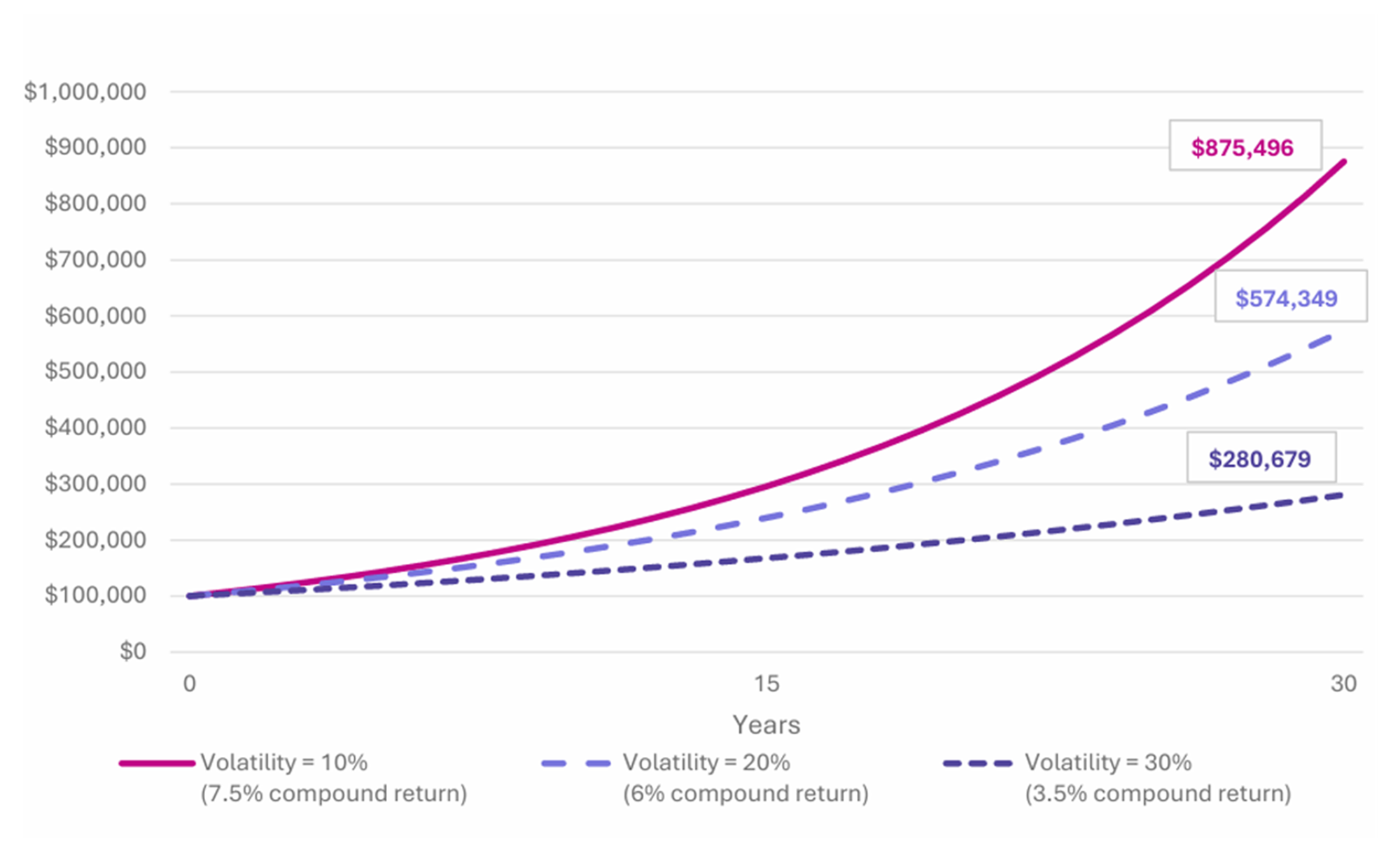
Note: For illustrative purposes only. Calculation does not take into account management fees, taxes, etc.
Diversification helps reduce risk
How do we move from the compound return of only 3.5% to a compound return of 7.5%, recalling that both portfolios have the same arithmetic return? Diversification. Reducing risk without sacrificing compound returns is the most widely recognized benefit of diversification. This principle operates at two levels.
First, within an asset class, owning a broad basket of securities helps reduce risk compared to owning only a small number of stocks. An investor who owns the entire asset class is less exposed to the misfortunes of any single company (i.e. the nearly 60% of firms that failed to outperform 1-month treasury bills since 1926).4
Second, across asset classes, combining investments in equities, fixed income, real assets, international markets, and private investments can further reduce overall portfolio risk. Because these asset classes respond differently to economic and market conditions, their returns don’t perfectly move in sync.
Diversification is derived from the fact that securities and asset classes do not all move in the same direction at the same time. When U.S. equities decline, bonds may hold their value or appreciate. When more expensive growth stocks struggle, less expensive value stocks or bonds may provide ballast. Similarly, real assets, like infrastructure and real estate, often respond differently to inflationary or geopolitical shocks than traditional stocks and bonds.
For a two-asset portfolio (a portfolio with only two holdings), total portfolio risk is a function of three components: the individual asset risk, the portfolio weight (how much of portfolio has allocated to each asset), and the correlation between the assets (how the two assets move in relation to one another). (See Appendix 2 for calculations.)
Assets that tend to move together offer little diversification benefit. If two assets are perfectly correlated, combining them does not reduce risk. However, as correlation declines, the portfolio’s total risk declines to something less than the risk of the sum of its components. This is where the magic can happen. As correlation decreases, the potential diversification benefit generally increases. When correlation is zero, risk reduction can be substantial. When correlation is negative, meaning the assets tend to move in opposing directions, the potential reduction may be even greater (see Appendix 2). In practice, most asset classes exhibit correlations ranging from positive to near zero, with some relationships occasionally turning negative.
Taking it a step further, investing risk is driven by two primary sources. The first source, systematic risk (or market risk), is the result of broad macroeconomic factors such as central bank policy, business cycles, and geopolitical events. Investors are compensated in the form of a risk premium, which provides a higher expected return above the risk-free rate. The extent to which an individual asset moves in response to the market is referred to Beta and will be discussed in greater detail in the next part of this series.
The second source of risk is unsystematic risk — also often referred to as idiosyncratic or company-specific risk — which is distinct to a company or industry. Highly competitive financial markets do not reward investors for taking on unsystematic risk in their portfolios. Unsystematic risk can be minimized through diversification. Said differently, portfolios with exposure to unsystematic risk — risk that could’ve easily been diversified away — do not have higher expected returns than portfolios with no unsystematic risk.
Figure 2 illustrates what happens to portfolio risk as the number of stocks in an underlying portfolio increases. The y-axis measures portfolio risk, while the x-axis shows the number of stocks in each portfolio. The volatility of the broad market is 15.8%. The area above 15.8% portfolio risk (dotted line) is unsystematic risk that declines with higher levels of diversification. The Raspberry curve shows declining portfolio risk from increasing diversification, which approaches but never crosses the market volatility floor.
Figure 2: Unsystematic Risk Shrinks as Portfolio Assets Grow
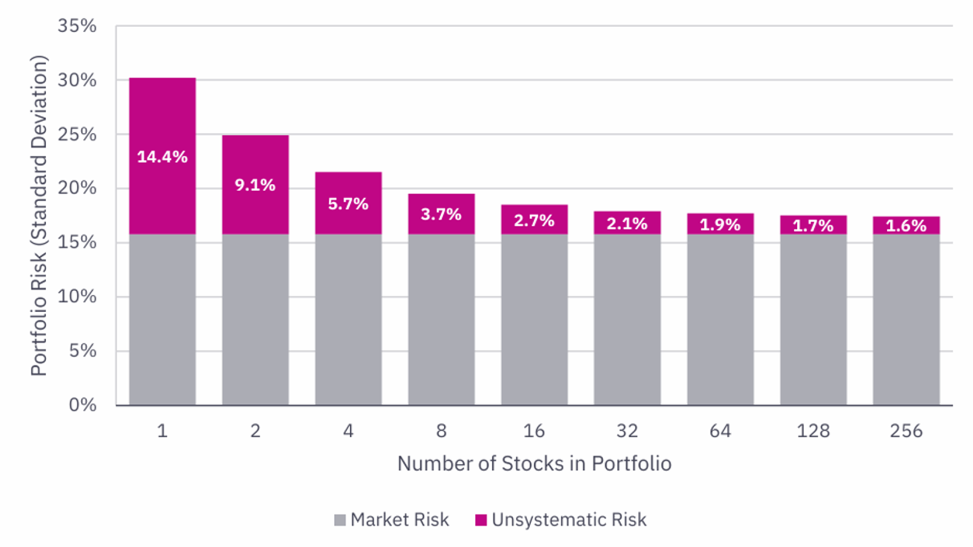
Notes: For illustrative purposes only. Results of 1,000 independent portfolios drawn at random from the S&P 500. Market risk is estimated as the annualized standard deviation of the equal-weight market portfolio.



Diversifying within and across asset classes allows the investor to get as much value as possible (in the form of returns) in exchange for what they pay (in terms of risk). By combining assets with different return drivers, investors can create portfolios that deliver a higher expected return for a given level of risk, or equivalently, a lower level of risk for a given expected return.
Diversification can increase compound returns
We have explained how diversification helps reduce risk and explored the destructive impact of volatility drag on compound returns, a critical driver of long-term wealth accumulation. We now turn to another important benefit of diversification: A portfolio with two or more imperfectly correlated assets will likely have a higher compound return than a simple average of the compound returns of the underlying assets within the portfolio. This phenomenon is known as the diversification benefit (or the rebalancing bonus) and it arises from the difference between the arithmetic and compound returns.
In a 1992 study, Nobel Prize-winning economist Eugene Fama and David Booth demonstrated how diversification affects both portfolio risk and compound returns.5 Their analysis began with a simple portfolio consisting of a single asset class with a compound return of 8% and a risk level of 20% (Figure 2). They then sequentially added additional asset classes, each with the same expected compound return (8%) and risk (20%).
Table 1 illustrates the results. A portfolio consisting of a single asset class has a risk level of 20% and a compound return of 8.00%. When a second asset class with the same return and risk characteristics is added, but with less-than-perfect correlation to the first, portfolio risk declines to 18.44% while the compound return rises to 8.30%. The addition of the second asset class reduces portfolio risk to a level below that of either individual asset class while simultaneously increasing the portfolio’s compound return above that of either asset class on its own. The same pattern continues as additional asset classes are added. As diversification broadens, the potential benefits of risk reduction and long-term compounding generally increase.
This is the same mathematical principle illustrated in Figure 1. Diversification transforms a concentrated portfolio with a compound return of 3.5% (represented by the purple dotted line) into a portfolio with a compound return of 7.5% and a risk level of 10% (represented by the raspberry dotted line).
Table 1. Diversification Benefit From Each Additional Asset Class Added to a Portfolio
| Quantity of Asset Class | Asset Class Risk (%) | Cumulative Portfolio Risk (%) | Asset Class Return (%) | Portfolio Compound (%) | Diversification Benefit (%) |
|---|---|---|---|---|---|
| 1 | 20 | 20.00 | 8.00 | 8.00 | 0.00 |
| 2 | 20 | 18.44 | 8.00 | 8.30 | 0.30 |
| 3 | 20 | 17.89 | 8.00 | 8.40 | 0.40 |
| 4 | 20 | 17.61 | 8.00 | 8.45 | 0.45 |
| 5 | 20 | 17.44 | 8.00 | 8.48 | 0.48 |
| 6 | 20 | 17.32 | 8.00 | 8.50 | 0.50 |
| 7 | 20 | 17.24 | 8.00 | 8.51 | 0.51 |
| 8 | 20 | 17.18 | 8.00 | 8.52 | 0.52 |
| 9 | 20 | 17.13 | 8.00 | 8.53 | 0.53 |
| 10 | 20 | 17.09 | 8.00 | 8.54 | 0.54 |
Source: For illustrative purposes only. Analysis based on findings from “Diversification Returns and Asset Contributions,” David G. Booth & Eugene F. Fama. Financial Analysts Journal, May/June 1993.
Once the portfolio holds 10 equally weighted asset classes, each with a compound return of 8% and risk of 20%, portfolio risk has fallen to 17.09%, nearly three percentage points below that of any individual asset class. At the same time, the portfolio’s compound return has increased to 8.54%, or 54 basis points higher than the return of any individual asset class. This increase in return is the diversification benefit: higher compound returns achieved through the reduction of volatility.
Over a 30-year investment horizon, this seemingly modest increase in return compounds into a meaningful wealth advantage. A $1 million portfolio growing at 8% annually would accumulate to approximately $10.1 million. The same portfolio growing at 8.54% would grow to approximately $11.7 million. The resulting $1.6 million difference is attributable to the higher compound returns made possible by risk reduction through diversification. As Harry Markowitz, the founder of Modern Portfolio Theory, famously observed, diversification is “the only free lunch in finance.”
The value of one basis point
Critics of broad diversification often point to diminishing marginal benefits. As shown in Table 1, the diversification benefit associated with adding a tenth asset class is just one basis point (0.01%) of additional compound return and four basis points (0.04%) of risk reduction. At first glance, these gains may appear insignificant. Yet this perspective overlooks an important question: why would an investor willingly accept higher risk and lower returns when a better alternative is available at little or no additional cost?
Even seemingly small improvements can translate into meaningful dollar amounts over time. For a $3 million portfolio invested over a 30-year retirement horizon, an additional one basis point of annual compound return results in approximately $9,000 of additional wealth. That’s nearly enough to cover a year of in-state tuition at a typical public four-year university or roughly five years of premiums for a high-quality Medicare Supplement plan.
Viewed this way, any portfolio that is less than fully diversified imposes a real and measurable cost on the investor. As long as the marginal benefits of additional diversification exceed the marginal costs, such as trading expenses, investors should capture every available diversification benefit.
Put differently, investors should seek to collect as many of finance’s “free lunches” as possible.
Diversification can support wealth over time
A third benefit of diversification is that it can increase the reliability of achieving the compound returns needed to help achieve and sustain our Economic Freedom.
Consider a 65-year-old retiree with $3 million in savings. She plans to withdraw 4% annually ($120,000) and increase those withdrawals by 3% each year to keep pace with inflation. Given her good health, she expects to live to age 90, meaning her portfolio must support her spending needs for at least 25 years. Her objective is straightforward: maximize the probability that her portfolio does not run out of money during retirement.
She is considering two very different equity portfolios. Portfolio A consists of a relatively concentrated collection of popular individual stocks with an expected return of 8% and a risk level of 30%. Portfolio B consists of a globally diversified stock portfolio. It has the same expected return of 8% but a substantially lower risk level of 12%.
Which portfolio more reliably supports her retirement goals? Table 2 summarizes the results of Portfolio A and Portfolio B:
Table 2. Probability of Running Out of Money in Retirement
| Portfolio A | Portfolio B | |
|---|---|---|
| Arithmetic Mean | 8% | 8% |
| Volatility | 30% | 12% |
| Compound Return | 3.5% | 7.28% |
| Probability of running out of money in retirement | 51% | 5% |
Notes: For illustrative purposes only. Calculations do not include taxes, management fees, etc. Results shown based on probability density of 10,000 Monte Carlo simulations of the compound return from specified distributions.
Portfolio A, with its 30% risk level, experienced portfolio failure in 51% of the simulations, meaning there was only a 49% probability that her assets would last through age 90. In effect, relying on Portfolio A amounts to little more than a coin flip, hardly an ideal foundation for retirement security.
Portfolio B produced dramatically different results. Despite having the same expected return, its lower risk profile resulted in a 95% probability of successfully funding her retirement through age 90. This substantial improvement is attributable entirely to the reduction in portfolio risk made possible through diversification.
Critics often argue that broad diversification dilutes wealth creation by sacrificing upside potential. In this example, the opposite is true. Although both portfolios have the same expected return, Portfolio A generated an average ending wealth of $7.9 million at age 90, while Portfolio B produced an average ending wealth of approximately $8.8 million. In other words, the more diversified portfolio generated nearly $1 million in additional ending wealth.
Far from limiting wealth creation, diversification enhances it. By reducing volatility and the resulting drag on compound returns, diversification not only increases the likelihood of financial success but also improves the amount of wealth accumulated over time. The result is a portfolio that is both more resilient and more productive, delivering a higher probability of meeting spending needs while simultaneously producing greater long-term wealth.
Lower risk, greater potential
Diversification is a fundamental driver for long-term investment success. Because wealth creation is concentrated among a small number of assets and future winners cannot be predicted with confidence, broad diversification can allow investors to participate in market growth while minimizing uncompensated risk. By reducing risk, diversification helps lessen the drag on compound returns, while enhancing long-term wealth accumulation. Importantly, diversification may improve the likelihood of achieving financial goals by helping investors build, preserve, and sustain wealth over time. For these reasons, broad diversification across and within global asset classes is how we help ensure that our clients do not overpay and achieve Economic Freedom.
APPENDIX
Appendix 1.
The relationship between arithmetic and compound returns is:
Compound return = Arithmetic return – [σ2/2]
Where:
σ2 = Portfolio variance
[σ2/2] is the volatility drag
As the portfolio variance (volatility squared) increases, the compound return decreases. The relationship between the volatility drag and compound returns is quadratic (exponential in behavior). Doubling the portfolio’s volatility quadruples the drag.
σρ2 = wa2σa2 + wb2σb2 + 2wawbσaσbρab
The Portfolio variance (σρ2) of a portfolio with two assets is:
Where:
wa = weight of asset A
wb = weight of asset B
σa = standard deviation (square root of the variance) of asset A
σb = standard deviation (square root of the variance) of asset B
ρab = correlation coefficient of asset A and B (ranging from -1 to +1)
When ρab is <1, the last term declines. When ρab is <0, the portfolio’s overall risk is lower than the sum of the individual risks of assets A and B.
1 “Do Stocks Outperform Treasury Bills?” Journal of Financial Economics, 2018.
2 “One Hundred Years in the U.S. Stock Markets.” SSRN, March 20, 2026
3 For purposes of this discussion, we use the terms “risk” and “volatility” interchangeably. Mathematical terms, such as variance, co-variance, and standard deviation, are more precise measures used by financial professionals and economists to measure different dimensions of risk. Those terms are used in the appendices and figure notes when applicable.
4 “One Hundred Years in the U.S. Stock Markets.” SSRN, March 20, 2026
5 “Diversification Returns and Asset Contributions.” Financial Analysts Journal, May/June 1992.
All expressions of opinion reflect the judgment of the author as of the date of publication and are subject to change. Some of the research and ratings shown in this presentation come from third parties that are not affiliated with Mercer Advisors. The information is believed to be accurate but is not guaranteed or warranted by Mercer Advisors. Content, research, tools and stock or option symbols are for educational and illustrative purposes only and do not imply a recommendation or solicitation to buy or sell a particular security or to engage in any particular investment strategy. All investment strategies have the potential for profit or loss. Diversification does not ensure a profit or protect against a loss. Economic factors, market conditions, and investment strategies will affect the performance of any portfolio and there are no assurances that it will match or outperform any particular benchmark. Hypothetical examples are for illustration purposes only and do not represent an actual investment. Actual investor results will vary.
For financial planning advice specific to your circumstances, talk to a qualified professional at Mercer Advisors.